Autonomous Underwater Vehicle (AUV-IITB)
About Team
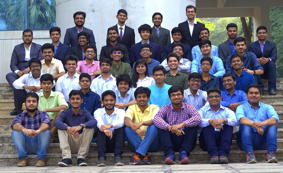
AUV-IITB comprises of highly enthusiastic and hard-working technocrats ranging from bright-eyed freshmen to driven senior undergraduates and tech-experienced post-graduates spanning various branches of engineering like Mechanical, Electrical, Software, Aerospace, Material Science and Civil at Indian Institute of Technology Bombay. The team works towards participating at AUVSI Robosub Competition, which is held annually in July at San Diego, California. The competition is a platform for students to display their skills in underwater robotics and build a connection with industries working along similar verticals. The competition demands designing and manufacturing of an autonomous underwater vehicle that can perform predefined tasks. This draws upon the expertise in the areas of engineering provided by the multifaceted team. Currently, we are a 40 membered team developing cutting edge technology for Autonomous Underwater Vehicles (AUV). The development of an AUV is a year-long process involving design, manufacturing, assembly, testing, integration, and competition preparation. In order to accelerate the development of MATSYA, our team is structured into three sub-divisions viz Mechanical, Electrical, and Software. Every year the team puts in 30,000 man-hours for the development and integration of our AUV MATSYA.
Achievements
| Runners-up at Robosub 2016 (amongst 50 international teams) |
| Finalists in Robosub 2017 |
| Winners at NIOT SAVe 2019 (amongst 14 national teams) |
| Semi-Finalists in Robosub 2018 and 2019 |
| Winners at NIOT SAVe 2016 (amongst 14 national teams) |
| Best performance by an Asian AUV at Robosub 2016 |
| Best performance by an Indian AUV at Robosub 2012-2017 |
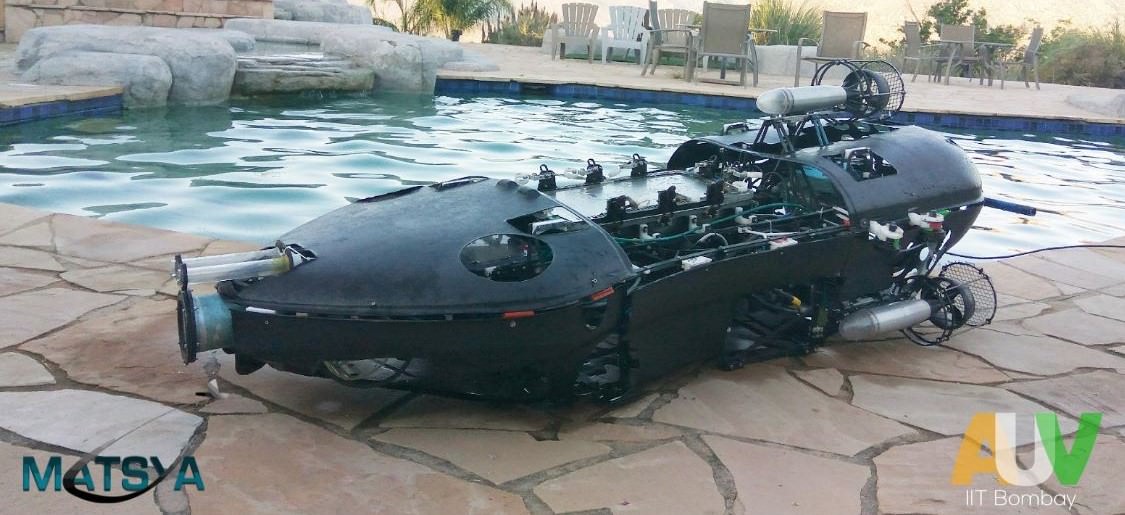
Matsya
My role in the team
Second Year
In my second, my work was to complete the advance and complicated development goals. The second-year students were expected to mentor the newly joined freshmen and help them to learn about the codebase. We also had a task to design the different aspects of the architecture, which ensured that everyone would have an idea about the overall working of the code.
ML Databasing Tool
Machine Learning is the new craze these days. It’s a very magical field, and you can get a task done which was never before imagined to be possible. We traditionally only used the classical image processing techniques for our vision package. It was pretty robust, for the detection of simple shapes and colors such as a red buoy, square cut out, etc. But when the competition demanded us to identify complicated images, we opted to use the machine learning algorithms. One of the most frustrating parts of machine learning is to annotate the images and create a dataset for training the model. My task was to create a handy and easy to use tool which will make this job more manageable.
Ml Tool is a databasing tool, which helps to create bounding boxes and label them. It takes a video as its input and enables us to mark the boxes frame by frame in the video. Since we had an abundance of video log, there was no shortage of data. This was made entirely from scratch using pygames.
Design
The Design of this Tool is something that I’m quite proud of. From the very beginning, I followed the modular design principle by splitting my code into different files, classes, etc. Pygames provides an elementary set of GUI functions. This is good if you want to have granular control. I created classes of each GUI element with functionality built into the class. This enabled me to quickly stitch together the interface without cluttering the original code too much.
Here are the different layers of the ML Tool.
| Text Class | Any text that you see on screen in pygames has to be rendered from a font class and then blit it onto a surface. Also, we have to take care of the position and size of the text. The text class handles all this like a charm while providing a handy way to draw text on the screen in just a single line of code. |
| Button Class | All the clickable elements that you see in the Tool belong to the button class. This class provides functionalities like drawing a button on the screen, having a background color or image for the button, status indicators for toggle buttons, shortcut key handler, click handler. All these features make adding buttons quite easy. |
| Box Class | This feature was added in the later version of the Tool. From the feedback received by the users, many complaints about the way boxes were handled in the Tool. To tackle that the Box class was added which provided the functionalities like a clear indication of the box which is selected for editing, ability to resize a box after it was drawn, edit box by dragging the corners, etc. |
| Subroutines | The Subroutines provided a different separate screen for a particular task. The “Box drawing area” is a subroutine inside the main while loop. In the future, we can extend the ability of the Tool by merely introducing more subroutines. |
| Video Handler | This layer takes care of how video files will be read, stored, and managed in the program. Right now, the program simply reads the whole file, and stores it an Array and then pass it to the main loop. In the future, support for different video formats and databases can be added just by editing this layer. |
| Popup Messages | In every GUI, feedback is essential. The user should know with certainty that the button is clicked or not; his files are saved or not. I developed a simple system to take care of this. Just using an array and two simple functions, I introduced the functionality to display a message text on the screen from anywhere you like in the code only by adding a single line. |
| Database handler | This is a simple layer that handles the way the boxes will be saved. We can change this layer to save the data better suited for our machine learning model. |
Sensor Fusion for Localization using Extended Kalman Filter
This was a research project, in order to check the feasibility of implementing a Kalman filter-based localization algorithm. Here is a synopsis of what I learn. This article contains a brief introduction to Kalman filter, the problem of POSE estimation in underwater vehicles, and an approach to implement extended Kalman filtering for the same. There are also details about the outputs of different sensors like IMU, DVL, and how to use the data from the sensors.
POSE Estimation Problem
What is the POSE estimation problem?
The estimation of position and orientation of a body in some space with respect to some frame of reference is called the POSE estimation problem.
This is a general problem in the field of autonomous robotics. Every autonomous robot needs to have some kind of sense of its surroundings and awareness about its position with respect to other objects in the real world. This especially a really hard problem for the underwater vehicles due to the lack of cheap ranging sensors underwater. To overcome this problem, we use data from several sensors to estimate the POSE of the robot and then fuse the estimate using filtering algorithms to get a better estimate than any sensor could produce on its own.
In this article, we will be discussing the Kalman filter to fuse the data from the different sensors and get a better estimate of the position and orientation of the bot.
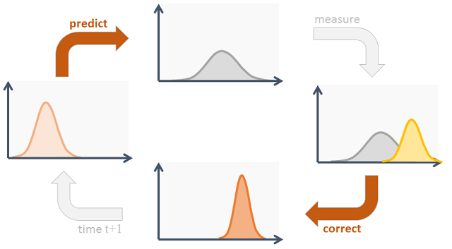
Kalman Filter
Probably the best-studied technique for implementing Bayes filters is the Kalman filter(KF). The Kalman filter was invented in the 1950s by Rudolph Emil Kalman, as a technique for filtering and prediction in linear systems. The Kalman filter implements belief computation for continuous states. It is not applicable to discrete or hybrid state spaces(i.e. when the system is non-linear).
The Kalman filter represents beliefs by the moment’s representation: At time t, the belief is represented by the mean μt and the covariance Σt
In the above mentioned formula,
- μt - State space at time t.
- Σt - Covariance matrix at time t.
- ut - Control space at time t.
- zt - Measurement space at time t.
- At - How the next state is depended on the previous state at time t.
- Bt - How the next state is depended on the control signals at time t.
- Ct - How the next measurement is dependent on the current state at time t.
- Rt - Covariance related to the State transition at time t
- Qt- Covariance in the measurement at time t
| State Space | This is a matrix that can completely(fully) describe the state of the robot. For e.g. a car can be fully defined by its position, velocity, acceleration, and towards which direction it is facing. Let’s say we require n variables to fully describe the state of the vehicle then the state space would be an nx1 matrix. |
| Control Space | This is a matrix that contains all the control parameters by which our bot is controlled. For e.g in the case of the car, the amount of acceleration and brake pedals pressed can be the control parameters. Let’s say we have m control variables, then the control space would be a mx1 matrix. |
| Measurement Space | This is a matrix that contains all the different variables which we can measure. For e.g. in the case of the car, we can have the velocity, position of the car from the GPS, etc. Let’s say we have k measurable variables, then the measurement space would be a kx1 matrix. |
| Covariance matrix | This is the covariance matrix of the state space. The shape of this matrix is nxn. |
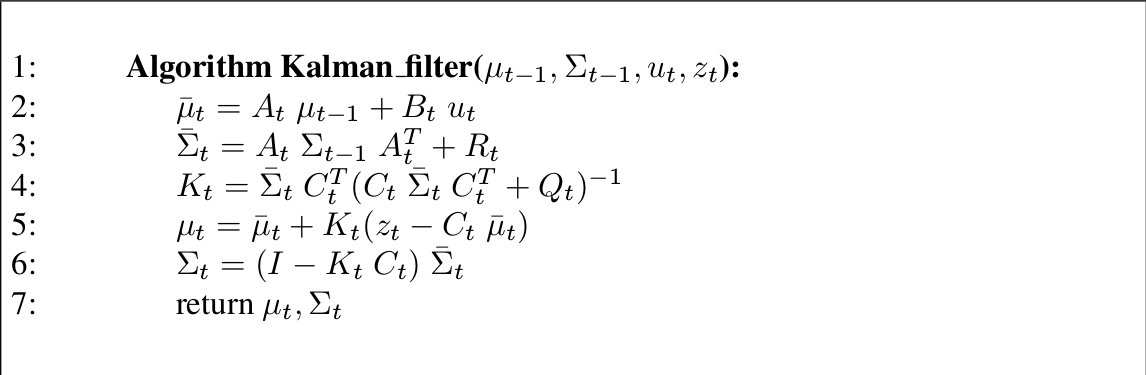
| A & B matrices | These matrices are used to predict the next state, using the previous state and the control data. The A matrix models the relationship between the previous state to that of the next state. Hence the shape of this matrix is nxn. The B matrix models the relationship between the control data and the next state, hence the shape of this matrix is nxm. Hence using the previous state can the control data we can predict the next state of our bot. This is accomplished by the first two equations of the algorithm mentioned in the above picture. These steps are also known as prediction steps. |
| C Matrix | This matrix denotes what the measurement should be given the current state space. Hence the shape of this matrix is kxn. |
| R & Q matrices | These are the covariance matrices for the state and measurement spaces respectively. These help to model the noise in the system. The shape R matrix is nxn, and the shape of the Q matrix is kxk. |
For more details on this, you can refer to the book on “Probabilistic Robotics”, This book covers the various filtering methods in detail, and this article was greatly referred from this book.
Extended Kalman Filter
Even though Kalman filters are very good for a wide range of applications. They can be used for nonlinear systems, i.e. the system in which the next state is given by some non-linear function of the previous state and control data. Also, the measurement can be a nonlinear function of the state.
The above is the model equations for the EKF model. And the algorithmic equations are as follows.
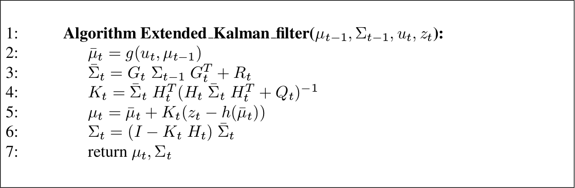
Note:- A quick trick to grasp Extended Kalman filters once you are comfortable with the linear Kalman filter is, just replace the A matrix with G and C matrix with H in the linear equations to get the extended Kalman equations.
Reverse Engineering the proprietary NI-DAQ Drivers
The Problem
One of the tasks in the Robosub competition is to locate the underwater pinger. For this, we have four hydrophones on the vehicle. We use the Time Difference Of Arrival (TDOA) approach to triangulate the location of the pinger. For doing this accurately we need to collect a lot of samples from the hydrophones. Hence to accomplish this we use the National Instruments Data Acquisition (NI-DAQ). Using the device we collect a million samples in two seconds.
The main problem with the NI-DAQ is that the drivers for it are only available in windows. But the entire stack of our vehicle runs on Ubuntu. Earlier we had to use windows inside a virtual machine and then connect to the program inside the VM using a socket. This solution worked for the most part, but when running the VM with all the other programs it uses to randomly crash. This caused a lot of problems as the system is autonomous and has cost the team competition due to the crashing of VM in the finals.
The Solution
One of the craziest solution we had of this problem was to reverse engineer the proprietary drivers of the NI-DAQ and write them in ubuntu. The DAQ connect to the vehicle via ethernet and used the TCP protocol for communication. The idea was to run the driver program normally in windows and capture the packets by monitoring the network using Wireshark. Then send those exact same packets from ubuntu. This was a replay attack.
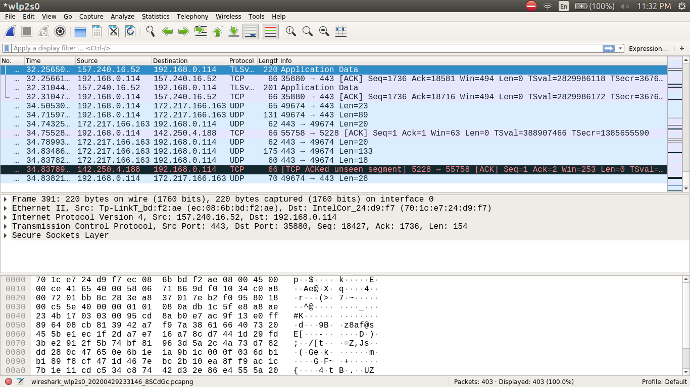
This was quite a tedious job, wherein we had to figure out which were the actual packets that matters. Also, there were multiple connections on different sockets and the timing of the packets in each socket was to be considered. We simply wrote a program that can read a pcap file and convert it into c++ format variables which could be then easily imported into the driver program and replayed.
First Year
I joined the team in September of 2018, in my first year, after clearing a two-stage selection process, which comprised of a written test and interview round. I learned a lot of new things in my first year as a part of this team, like ROS, git, bash, etc. Here is a list of the task I accomplished.
Databasing with HDF5
This was my first task in the team. The purpose of this task was to get me familiarised with the work of our code and ROS framework. The vehicle has four hydrophones, which collects the underwater acoustics data. This data is analyzed in software to locate sound sources inside the water.
The task was to create a program that will take the raw data collected by the acoustics driver and then convert and store it in the HDF5 database. The idea was to use the compression of the HDF database and save some space while saving the readings. We collected a million samples in two seconds from each of the four hydrophones. This created around 64 Mb of raw data, and it adds up quickly if the acoustic program is running for a long time.
Here is the description of the program and my approach. Internal Link to the file
# $Id: hdf5write.py$
# Author: Parth Patil <parthvin@gmail.com>
# Copyright: AUV-IITB 2017

"""
This program writes simple hdf5 files

It takes the bin files i.e. the raw data received from hydrophones
and converts them to text files through fft (present in auv_acoustics)
then it writes the text file to a hdf5file in table format

The module contains the following
Functions:

- 'init' :takes all the agruments recieved and put them in a map
          named variables

- 'runfft' :calls fft and converts the bin to text file
            and saves the final 'YAW' and 'PITCH' in
            final_data and return final_data

- 'lines_infile' :takes the text filename name and returns
                  number oof lines present in the text file

- 'create_file' :opens a hdf5file if it exists or creates a new
                 new hdf5file in /HDF5Files directory and returns
                 h5py.File object

- 'data_write' :take the variables map,hdf5file,and final_data &
                writes the data from the text file to a hdf5file
                and add the final data as attribute to the dataset
"""
Overall this was a pretty simple task, but it played an important role in paving my way in the auv_acoustics package.
Auto Frequency Detection
Aim
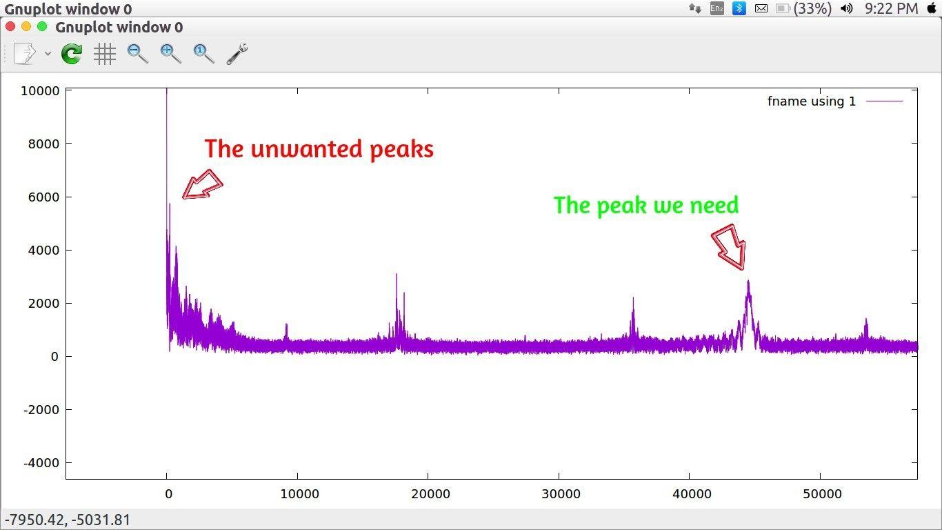
The vehicle gets input from the Hydrophones, which in the form of a sound wave with respect to time. This wave is a superposition of many waves of different frequencies. The aim was to identify the frequency of the pinger present in the water and apply filters around that frequency to reduce the noise from the surrounding. For this, I have to create a program that will detect the frequency of the incoming sound source.
Approach
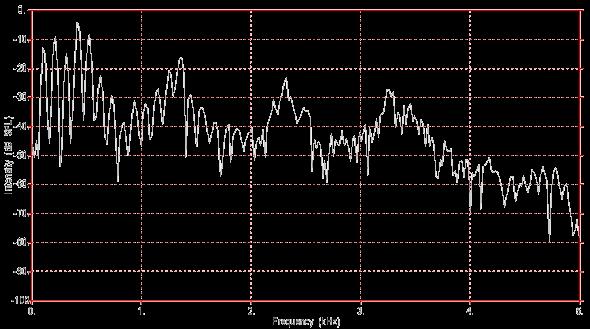
The method to detect the most dominant frequency present in the signal was to simply take a Fourier Transform (FT) of the signal, then get the Power Spectrum of the FT and then look for the maximum amplitude present in the Power Spectrum.
The Fourier transform decomposes a function of time (a signal) into the frequencies that make it up, in a way similar to how a musical chord can be expressed as the frequencies (or pitches) of its constituent notes. The Fourier transform of a function of time itself is a complex-valued function of frequency, whose absolute value represents the amount of that frequency present in the original function, and whose complex argument is the phase offset of the basic sinusoid in that frequency.
The Power Spectrum of a time series describes the distribution of power into frequency components composing that signal. According to Fourier analysis, any physical signal can be decomposed into several discrete frequencies, or a spectrum of frequencies over a continuous range.
Implementation
To implement this, I used the fftw library in c++ and NumPy in python.
I first had to store the data in arrays. The incoming data is discrete, so I used the DFT(Discrete Fourier Transform) functions from the libraries. Then after applying the DFT, we get a complex array. Every value in the array corresponds to the intensity of the component of frequency present in the incoming sound source.
Note:- Since the incoming data consists only of real numbers, we consider only half of the DFT since it would be symmetric. You can read more that over here
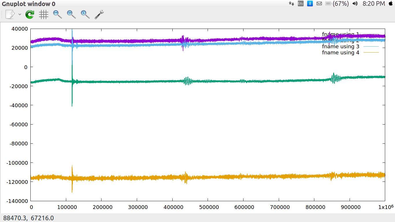
To find the element in the complex array with the maximum intensity, I computed the power spectrum of the data (i.e., basically calculating the modulus of complex numbers). While doing this, I realized that in the data, after applying FFT and computing power, it was found that there was a peak at the very starting and very end of our data. Like e.g. After using DFT on 106 data points and then computing power spectrum of 0.5x10⁶ data point the value of power spectrum around 10000 data points at the start and the end would be higher than that of the actual peak that we have to detect (i.e., the peak corresponding to the frequency of the sound source). So to overcome this problem, we can straight away neglect those values since we know that our frequency will not fall in that range
This is a code snippet for implementation:
file_path = req.filepath
data  = data_read(file_path)
fft_data = apply_fft(data)
powr_spec = power_spec(fft_data)
filter_intial(powr_spec)
detected_freq = int(auto_freq_detect(powr_spec))
save_data(powr_spec)
Here the data_read function reads the data from a file or from a ros topic and returns the array of the incoming signal. The apply_fft function applies the DFT on the data. The power_spec computes the power spectrum of the fft_data generated. And the filter_inital set the value of initial and ending conflicting values to zero. And the auto_freq_detect find the maxima compute its corresponding frequency and return it. You can refer to the detailed code here (Internal link) .
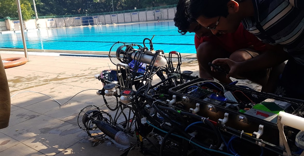
Learning to test the vehicle is an important skill that you have to learn as a part of the software subdivision. Testing teaches us that “Things don’t work as we expect them to work”. The code we write may seem to be perfect, but once we run it inside the pool along with everything else, it may fail. And to win the competition, it is utmost necessary to have a robust testing system.
For testing our programs, we first have to run them in the simulator and check if everything is running smoothly, and there is no breaking error in the code. We call this “Simulator Testing”. This ensures that if the code runs on the actual vehicle in the pool, it won’t do something crazy and damage the vehicle. This step also reduces the time of debugging at the pool as we can quickly test the programs on our laptop at our comfort.
The next step of testing is to take the vehicle inside the pool, and recreate the task environment, to test the working of the vehicle. In this, we not only have to learn to debug the software code but also understand the mechanical and electrical aspects of the vehicle and get a grasp of which component might have failed. This process enhances the understanding of how all the parts in the vehicle work.


Web Based Testing Interface
The Problem
After doing the testing, I realized there were some flaws in our process. One such issue was the lack of any intuitive interactive testing interface. This prevented people who are not comfortable with terminals from testing the vehicle. Even for testing some small things in elec-stack, we use to have someone from the software subdivision to run the terminal commands. To tackle this, we needed a Graphical Interface that was easy to use and understand.
Overview of the Approach
I chose to have a web-based interface because running a GUI is a somewhat cumbersome task, and we use LAN to connect to the vehicle while testing. Hence to access the GUI running on the Matsya, we would need to do SSH into the vehicle using Xterm, and on low bandwidth, it runs quite awfully. Also, one more problem was that not everyone in our team has Linux installed, as the Mechanical subdivision does most of their work on heavy software in windows. Hence opting for a web-based interface was an obvious choice as it can run on low bandwidth and would be independent of the operating system of the client.
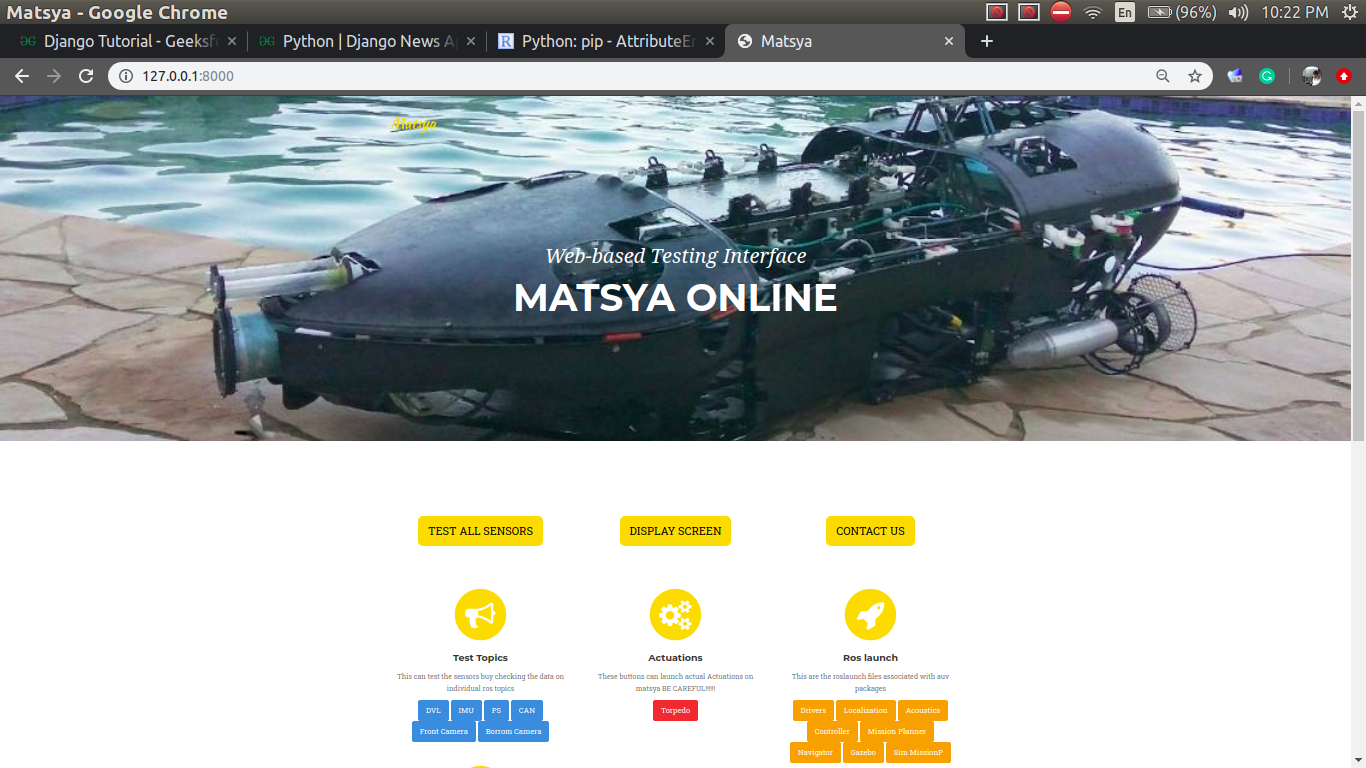
I used the Django server in the backend to serve the website. The front-end was created using Jekyll as a static web page, and then it was edited to fit the Django template engine. I also integrated the ROS framework with Django to open the door of ros commands to the interface. This enables the interface to do things like checking the sensors, shooting torpedos, controlling the arm, etc. Apart from these django-sockets was used to handle the asynchronous request from the client; this enabled things like reading the ros messages from ros topics, live remote terminal, remote display, and control.
Features and Design of the Testing Interface
| Django Backend | As mentioned earlier, Django was used in the backend; it provides a lot of functionalities. It handles a lot of networking for you. Hence we could just focus on the core utility part. I made two Django apps, and one was the home_page, and the second was ros_helpeer. The first app handled all the simple synchronous requests. The second app dealt with the complicated async requests like reading from a ros topic or displaying the contents of the screen on the interface. |
| Modular Design | For the very beginning, I kept in mind the modular aspect of the interface. Each button you see on the screen above is just a Django model. Hence adding a new button is just as simple as visiting the admin page of the website and customizing the button according to your need. You can even change what action a particular button performs quickly in the admin page. This enhances the interface such that one doesn’t also have to change the source code to make changes in the interface. This makes it self-sufficient. |
| Remote Command Execution | Many times in testing, one would like to do something which is quite task-specific, for this circumstance, one would wish to have a terminal available to them. This feature exactly does that. It provides a remote terminal, where you can type a single command and also look at it’s output. The output of the command also gets updated asynchronously. |
| Screen Casting and Remote Control | This is one of the feature I’m quite proud of. You can imagine this feature to be a simple version of Teamviewer or Anydesk. It gives the user ability to view the screen of vehicle at the same time enabling the mouse and keyboard control. The display that you see on the website is clickable, and you get a textbox to enter your keyboard presses. This is a very helpful feature if you want to run programs with GUI. |
| Monitoring Ros topics | One of the frequently used feature while testing is to monitor the rostopics and see if everything is working fine. I replicated this using the interface. A socket connection is made whenever the user chooses to monitor a topic, and when a message is received, the data is sent to the front-end via a WebSocket. |
| Django-sockets | One of the significant features of the project was its ability not only to handle synchronous requests but also connect to the front-end via asynchronous means. For this, I used a library django-sockets which uses workers and consumers to serve the webpages continuously. |